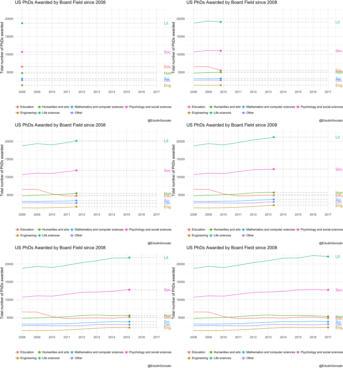
Finally I got myself into the #tidytuesday. This project, promoted by R for Data Science, aims to enhance the manipulation and visualisation skills among the R community by the exploratory analysis of a raw new dataset that is posted on a weekly basis. Apart from improving the #RStats skills, the idea of this project is to enable connections amongst the #Rstats community, explore other´s work and get feedback.
The data for this week consisted of sample of PhDs awarded by field in the US. The dataset is relatively small with just 5 variables that give information about the broad, major and main field, the year of the award and the number of PhDs awarded.
library(tidyverse)
library(gganimate)

grads = read_csv("https://raw.githubusercontent.com/rfordatascience/tidytuesday/master/data/2019/2019-02-19/phd_by_field.csv")

glimpse(grads)
## Observations: 3,370
## Variables: 5
## $ broad_field <chr> "Life sciences", "Life sciences", "Life sciences", "…
## $ major_field <chr> "Agricultural sciences and natural resources", "Agri…
## $ field <chr> "Agricultural economics", "Agricultural and horticul…
## $ year <dbl> 2008, 2008, 2008, 2008, 2008, 2008, 2008, 2008, 2008…
## $ n_phds <dbl> 111, 28, 3, 68, 41, 18, 77, 182, 52, 96, 41, 32, 44,…For my representation I want to calculate the number of students for each year in each broad_field for each year. Also, I create a variable (lab_clean) with shorter names for the broad fields. It will be helpful for the representation afterwards.
check = grads %>%
  group_by(broad_field, year) %>%
  tally(n_phds) %>%
  mutate(lab_clean = case_when(broad_field == "Education" ~ "Edu.",
                               broad_field == "Humanities and arts" ~ "Hum.",
                               broad_field == "Mathematics and computer sciences" ~ "Sci.",
                               broad_field == "Engineering" ~ "Eng.",
                               broad_field == "Life sciences" ~ "Lif.",
                               broad_field == "Psychology and social sciences" ~ "Soc.",
                               broad_field == "Other" ~ "Oth."))

head(check)
## # A tibble: 6 x 4
## # Groups: broad_field [1]
## broad_field year n lab_clean
## <chr> <dbl> <dbl> <chr>
## 1 Education 2008 6561 Edu.
## 2 Education 2009 6528 Edu.
## 3 Education 2010 5287 Edu.
## 4 Education 2011 4670 Edu.
## 5 Education 2012 4803 Edu.
## 6 Education 2013 4934 Edu.The visualisation is just a combination of geom_line() and gganimate.
ggplot(check, aes(year, n, group = broad_field, colour = broad_field)) +
  geom_line() +
  geom_segment(aes(xend = 2017, yend = n), linetype = 2, colour = 'grey') +
  geom_point(size = 2) +
  scale_x_continuous(breaks = c(2008:2017)) +
  geom_text(aes(x = 2017.5, label = lab_clean), hjust = 0) +
  transition_reveal(year) +
  coord_cartesian(clip = 'off') +
  labs(title = 'US PhDs Awarded by Board Field since 2008',
       y = 'Total number of PhDs awarded',
       x = " ",
       caption = "@EdudinGonzalo") +
  theme_minimal() +
  theme(legend.position = "bottom",
        plot.margin = margin(1.5, 1, 1, 1.5),
        legend.title = element_blank())
It seems that the number of PhD graduates in Humanities, Education, Sciences and Engineering have remained stable over time. Social and especially life sciences, however, have increased the amount of postgraduates since 2008.
Find the code on my Github repository.